Chat Spam Classifier - Part 2 - The Classifier

This is the second part of a series on spam classification.

Part 1: Labelling Training Data
Part 2: The Classifier
Part 3: Streaming Classification (TODO)
Part 4: Visualization (TODO)

The classifier is an ensemble of many classifiers, who’s output is the input to a single blender. Blending is also called stacking of stacked generalization in some literature. The blender is a simple logistic regression algorithm that will form the final prediction. Most algorithms used comes from Scikit-learn, but TensorFlow and XGBoost are also used.

First we need to preprocess the data to get numerical values we can operate on. Here we’re using a short pipeline consisting of a stemmer, TF-IDF vectorizer and a dense transformer. Since some of the classifiers don’t work on sparse data we want dense data:

transformers = {
    TFIDF: StemmedTfidfVectorizer(stemmer, min_df=1, stop_words='german', decode_error='ignore'),
    DENSE: DenseTransformer()
}

The stemmed vectorizer is a combination of a stemmer and TF-IDF vectorizer:

class StemmedTfidfVectorizer(TfidfVectorizer):
    def __init__(self, stemmer, **args):
        super(StemmedTfidfVectorizer, self).__init__(args)
        self.stemmer = stemmer

    def build_analyzer(self):
        analyzer = super(TfidfVectorizer, self).build_analyzer()
        return lambda doc: (self.stemmer.stem(w) for w in analyzer(doc))

The DenseTransformer looks like this:

class DenseTransformer(TransformerMixin):
    def transform(self, X, y=None, **fit_params):
        return X.todense()

    def fit_transform(self, X, y=None, **fit_params):
        self.fit(X, y, **fit_params)
        return self.transform(X)

    def fit(self, X, y=None, **fit_params):
        return self

Vectorization (Vector Space Model) is a technique for representing text as numerical vectors. This is useful for us since the classification algorithms used operate on numerical data. TF-IDF stands for Term Frequency, Inverse Document Frequency. TF-IDF is a way to find important words to the document relative to the complete corpus. For an introduction on how VSM and TF-IDF works I refer to Christian Perone’s introduction, both part 1 and part 2.

The ensemble contains the following 8 classifiers for the first layer. The parameters comes from cross-validation using scikit-learn’s GridSearchCV:

classifiers = {
    BAYES: MultinomialNB(alpha=0.02),
    LOG_SAG: LogisticRegression(penalty='l2', solver='sag', C=100, max_iter=250, n_jobs=-1),
    TENSOR_DNN: TensorFlowDNNClassifier(hidden_units=[10, 20, 10], n_classes=2, steps=1600, learning_rate=0.08, optimizer='Adagrad', verbose=0),
    FOREST: RandomForestClassifier(n_estimators=500, max_depth=100, verbose=0, n_jobs=-1, oob_score=True),
    SVC: LinearSVC(penalty="l1", dual=False, tol=1e-3),
    PERCEPTRON: Perceptron(n_iter=50),
    PASSIVE_AGGRESSIVE: PassiveAggressiveClassifier(n_iter=25, C=0.05, n_jobs=-1),
    XGBOOST: XGBoostClassifier(eval_metric='auc', num_class=2, nthread=8, eta=0.1, num_boost_round=100, max_depth=6, subsample=0.6, colsample_bytree=1.0, silent=1),
}

The second layer of the classifier is the blender. The blender predicts the true class from what the classifiers output:

blenders = {
    BLEND_LOG_LINEAR: LogisticRegression(C=15, penalty='l2', max_iter=150, n_jobs=-1, solver='sag'),
}

Here we can have many blenders and use majority voting as the third layer. Testing this did not increase the accuracy enough to justify the added complexity for us. A blending ensemble looks like this:

spam-levels

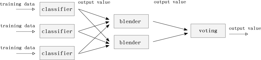
Now we can start to train the classifiers. If you have enough memory you could train some, or all, in parallel. Here we train them in sequence:

@staticmethod
def fit(X, y):
    X = Classifier.pipeline.fit_transform(X, y)

    for name, clf in Classifier.clfs:
        start = time.time()
        clf.fit(self.X_train, self.y_train)
        print('[%s] fitting took %.2fs' % (name, time.time()-start))

Before we can begin training, we need to initialize the transformers, classifiers and blenders:

@staticmethod
def train_classifier(data=None, validate=False):
    Classifier.set_transformers()
    Classifier.set_clfs()
    Classifier.set_bclfs()
    Classifier.train_model(data=data, validate=validate)
    Classifier.trained = True

@staticmethod
def set_clfs():
    Classifier.clfs = [
        (Classifier.BAYES, Classifier.classifiers[Classifier.BAYES]),
        (Classifier.LOG_SAG, Classifier.classifiers[Classifier.LOG_SAG]),
        (Classifier.TENSOR_DNN, Classifier.classifiers[Classifier.TENSOR_DNN]),
        (Classifier.FOREST, Classifier.classifiers[Classifier.FOREST]),
        (Classifier.SVC, Classifier.classifiers[Classifier.SVC]),
        (Classifier.PERCEPTRON, Classifier.classifiers[Classifier.PERCEPTRON]),
        (Classifier.PASSIVE_AGGRESSIVE, Classifier.classifiers[Classifier.PASSIVE_AGGRESSIVE]),
    ]

@staticmethod
def set_bclfs():
    Classifier.bclfs = [
        (Classifier.BLEND_LOG_LINEAR, Classifier.blenders[Classifier.BLEND_LOG_LINEAR]),
    ]

@staticmethod
def set_transformers():
    Classifier.pipeline = Pipeline([
        (Classifier.TFIDF, Classifier.transformers[Classifier.TFIDF]),
        (Classifier.DENSE, Classifier.transformers[Classifier.DENSE]),
    ])

Here we’re using clfs, bclfs and pipeline instead of classifiers, blenders and transformers. This is because we want to replace these later when the classifier is running on Spark. What we want is the pre-trained models that the trainer has saved to HDFS.

The data variable in the train_classifier method is simple a pandas DataFrame:

def load_data():
    table = config.get(ConfigKeys.JDBC_TABLE, 'training')
    cursor.execute("select class, message from %s" % table)
    _data = cursor.fetchall()

    return pd.DataFrame({
        '0': np.array([d[0] for d in _data]), 
        '1': np.array([d[1] for d in _data])
    })

data = load_data()

Now we can finally begin training, see the train_model method below:

@staticmethod
def train_model(data):
    y = data[data.columns[0]]
    X = data[data.columns[1]]
    y = np.array(y).astype(int)

    X_train, X_valid, y_train, y_valid = train_test_split(X, y)

    if not Classifier.trained:
        Classifier.fit_classifiers(X_train, y_train)

    X_blend = Classifier.validate_classifiers(Classifier.clfs, X_train, y_train)
    Classifier.fit_blenders(X_blend, y_train)

    X_blend = Classifier.validate_classifiers(Classifier.clfs, X_valid, y_valid)
    Classifier.validate_blenders(Classifier.bclfs, X_blend, y_valid)

Here we use the training set for prediction. The predictions is what’s used as training data for the blenders. If you have enough data it would be better to split the data into three separate sets. Use the first set to fit the classifiers and the second set to predict using the classifiers. Use the predictions as training data for the blenders, and use the third set to validate the blenders. In practice it didn’t have a big impact on the accuracy for us by doing it this way. The accuracy was still higher than not using a blender. 50k samples were also a bit too small of a dataset to be able to split into three sets. In the future when we have more labelled training data we can switch over to using three sets.

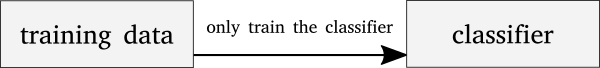
A quick visualization of this three-way split. We would first train the classifier on the training split:

training-split

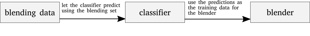
Then we validate the classifier using the second split, the ‘blending’ split. Use the predictions from the classifier as training data to the blender:

blend-split

Then we use the validation set to validate the classifier. Finally use the classifier’s output as input to validate the blender:

validation-split

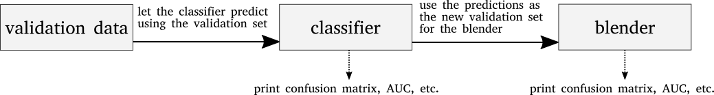
This way the blender gets trained on real training data that the classifier has not seen before. This makes the classifier train on one split and validate on two splits. The output of the second split is only used as training data for the blender. Now we can validate both classifier and blender with a split that neither has seen before.

Below is the validate and validate_blenders methods. We loop over the classifiers and aggregates the output:

@staticmethod
def validate_classifiers(classifiers, X, y):
    return Classifier.validate(classifiers, Classifier.pipeline.transform(X), y)

@staticmethod
def validate_blenders(classifiers, X, y):
    return Classifier.validate(classifiers, to_blend_x(X), y)

@staticmethod
def validate(classifiers, X, y, X_copy=None):
    def validate_classifier(_classifier, _name, X_valid, y_valid):
        if hasattr(classifier, 'predict_proba'):
            y_hat = _classifier.predict_proba(X_valid)[:, 1]
        else:
            y_hat = _classifier.predict(X_valid)

        score(y_hat, y_valid, name=_name)
        return y_hat

    y_hats = dict()
    for index, (name, classifier) in enumerate(classifiers):
        y_hats[index] = validate_classifier(classifier, name, X, y)

    y_hat_ensemble = score_ensemble(y_hats, y, len(classifiers))
    print_validation(y, y_hat_ensemble, X_copy)

    return y_hats

I won’t cover the score method, the only thing it does is printing some metrics.

Now we can combine this into a functional trainer:

data = load_data()
Classifier.train_classifier(data)

Now do some cross-validation until you’re happy with the accuracy you get. Then instead of splitting the data into a train and validation sets, retrain on one split. Use the second as training data for the blenders. This way we avoid the three-way split (not needed any more).

Next, store these models on HDFS so our Spark workers can download and use them across the cluster:

hdfs_path = config.get(ConfigKeys.HDFS_PATH, '/spam-models')
local_path = config.get(ConfigKeys.LOCAL_PATH, '/tmp/sf-models')

if not os.path.exists(local_path):
    os.makedirs(local_path)

# save models to hdfs so all workers can load them
hadoop = Hadoop(config.get(ConfigKeys.HADOOP_URL, 'http://localhost:50070'))
hadoop.delete(hdfs_path, recursive=True)
hadoop.upload(hdfs_path, local_path)

Above, config is a dictionary of configuration values read from Zookeeper. Since all workers need access to the config values it makes sense to get them from somewhere else. That way we don’t happen to have conflicting configurations spread out across the cluster. One way of getting these configuration values from Zookeeper is the following. env contains environment variables, either loaded from the yaml file or the shell:

def load_config(env):
    logger = logging.getLogger(__name__)
    zk_config_path = env.get('zk_config_path')
    zk_hosts = env.get('zk_hosts')

    zk = KazooClient(hosts=zk_hosts)
    zk.start()
    zk.ensure_path(zk_config_path)

    config = dict()
    for key, type in ConfigKeys.ALL:
        try:
            config[key] = type(zk.get('%s/%s' % (zk_config_path, key))[0])
        except NoNodeError as e:
            logger.error('could not get config key "%s" from zookeeper: %s' %
                         (key, str(e)))
            raise e

    logger.info('read configuration from zookeeper: %s', config)
    return config

The keys ConfigKeys.ALL can look something like this:

HADOOP_URL = 'hadoop-url'
HDFS_PATH = 'hdfs-path'
LOCAL_PATH = 'local-path'
JDBC_TABLE = 'jdbc-table'
JDBC_USER = 'jdbc-user'
JDBC_PASS = 'jdbc-pass'
JDBC_PORT = 'jdbc-port'
JDBC_HOST = 'jdbc-host'
JDBC_DB = 'jdbc-db'

ALL = [
    (HADOOP_URL, str),
    (HDFS_PATH, str),
    (LOCAL_PATH, str),
    (JDBC_TABLE, str),
    (JDBC_USER, str),
    (JDBC_PASS, str),
    (JDBC_PORT, int),
    (JDBC_HOST, str),
    (JDBC_DB, str),
]

Now that we have the pre-trained models stored in HDFS we can start looking a the Spark Streaming task.

Written on June 21, 2016